Showing posts with label Administration. Show all posts

Monday, October 5, 2009

Determine Which Indexes Are Not Being Used

Have you ever had the need to find out which indexes are actually being used?  If you are using SQL 2005 and greater, you are in luck.  SQL Server 2005 introduced a new dynamic management view that gives all the usage statistics, sys.dm_db_index_usage_stats (http://msdn.microsoft.com/en-us/library/ms188755.aspx).  What does this mean?  Well it means we can capture which indexes are being used and which ones are an administrative burden.  What’s the catch?  The catch is the usage statistics do not persist a SQL Server restart. The statistics will not be of much value after a server restart, so an option may be to insert the results of the view into a permanent table, for later analysis.  Let’s look at an example.

SELECT 
    QUOTENAME(s.name) + '.' + QUOTENAME(t.name) AS TableName,
    i.name AS IdxName,
    i.type_desc AS IdxType,
    ius.user_seeks,
    (ius.user_seeks*1.) / NULLIF((ius.user_seeks+ius.user_scans+ius.user_lookups),0) AS [%Seek],
    ius.user_scans,
    (ius.user_scans*1.) / NULLIF((ius.user_seeks+ius.user_scans+ius.user_lookups),0) AS [%Scan],
    ius.user_lookups,
    (ius.user_lookups*1.) / NULLIF((ius.user_seeks+ius.user_scans+ius.user_lookups),0) AS [%Lookup],
    ius.user_updates
FROM sys.indexes i
LEFT JOIN sys.dm_db_index_usage_stats ius
    ON  ius.object_id = i.object_id
        AND ius.index_id = i.index_id
        AND database_id = DB_ID()--Current DB
INNER JOIN sys.tables t
    ON t.object_id = i.object_id
INNER JOIN sys.schemas s
    ON t.schema_id = s.schema_id
WHERE
    t.type = 'U'
    AND t.is_ms_shipped = 0
ORDER BY ius.user_seeks + ius.user_scans + ius.user_lookups DESC
 

Note: I have used a left join.  If an index has never been used, it will not have an entry in sys.dm_db_index_usage_stats.

The columns that really drive this view are user_seeks, user_scans, user_lookups, and user_updates.  User_seeks represents the number of seeks on a given index, since SQL Server last started.  Likewise, user_scans and user_lookups represent the number of scans and the number of lookups respectively.  One of the most important columns is user_updates.  User_updates represents the number of inserts, updates, and deletes to the index. If you find your index in a scenario where the number of user_updates is greater than the number of seeks, lookups, or scans, you should consider dropping the index.  There is no magic number to dictate when an index should be dropped because of the maintenance overhead.  You should use your best judgment when dropping an index. 

There you have it a simplistic method to get the index usage details.  How else can this dynamic management view be used?  I leave this to you to find out, but I will leave you with one other use.

The other use for this view is to identify the most queried tables.  By looking at the index usage stats, we can deduce how often the table is queried. 

--Most Accessed Tables
SELECT 
    DB_NAME(ius.database_id) AS DBName,
    OBJECT_NAME(ius.object_id) AS TableName,
    SUM(ius.user_seeks + ius.user_scans + ius.user_lookups) AS TimesAccessed    
FROM sys.indexes i
INNER JOIN sys.dm_db_index_usage_stats ius
    ON  ius.object_id = i.object_id
        AND ius.index_id = i.index_id
WHERE
    ius.database_id = DB_ID()
GROUP BY 
    DB_NAME(ius.database_id),
    OBJECT_NAME(ius.object_id)
ORDER BY SUM(ius.user_seeks + ius.user_scans + ius.user_lookups) DESC

That is it.  I have provided two uses of sys.dm_db_index_usage_stats.  I hope this post will help you identify poorly performing indexes or you most active tables. 

Happy Coding.

Friday, August 7, 2009

Are all covering indexes created equal?

I have been getting a lot of questions regarding indexes over the past few weeks, so I thought I would make another post about indexes. In this post, I will be focusing on covering indexes.  A covering index is an index that covers all the columns for a given query.  A covering index can be created by either, adding the columns to the index key, or by adding the columns to the include clause of the create index statement. I will focus on the key differences between adding columns to the index key and adding columns to the INCLUDE clause.  I will look at the differences in size, statistics, and the execution plan.

Let’s get started by creating our test table.

USE [tempdb]
GO
 
SET NOCOUNT ON;
GO
 
IF EXISTS(SELECT 1 FROM sys.tables WHERE NAME = 'TestData')
BEGIN
    DROP TABLE dbo.[TestData];
END
GO
 
CREATE TABLE dbo.TestData(
RowNum INT PRIMARY KEY,
SomeId INT,
SomeCode INT
);
GO
 
INSERT INTO dbo.[TestData] (
    [RowNum],
    [SomeId],
    [SomeCode]
) 
SELECT TOP 1000000 
    ROW_NUMBER() OVER (ORDER BY t1.NAME) AS RowNum,
    ABS(CHECKSUM(NEWID()))%2500+1 AS SomeId, 
    CASE 
        WHEN ROW_NUMBER() OVER (ORDER BY t1.NAME) % 2 = 0
        THEN 1
    ELSE 0
    END AS SomeCode
FROM 
    Master.dbo.SysColumns t1,
    Master.dbo.SysColumns t2
GO

Now that we have our test table, I will create a covering index using the INCLUDE clause.

CREATE INDEX ncl_idx_TestData_Cover1 ON dbo.TestData(SomeID) INCLUDE(SomeCode);
GO

I will issue a simple query to select data from the table, using the new index.

SELECT 
    someid,
    somecode
FROM dbo.[TestData]
WHERE
    someid = 500 
    AND somecode = 1

The results of this query are inconsequential for our purposes, so I will not post them here; however, I will post the key attributes of the execution plan.

image 

The above screenshot shows that our covering index is used.  The primary thing to note here is deviation between the actual and the estimated number of rows. I will get into why these numbers deviate later in the post.

Let’s have a look at the space consumed by the index.  I will  issue a system stored procedure called sp_spaceused to obtain the space consumption details.

EXEC sp_spaceused 'dbo.Testdata' 

image

As you can see from the screenshot above, our index size is 18008 KB or  17.58 MB = 18008 / 1024. Now that we have our index size, let’s look at the statistics. I will be using the DBCC command show_statistics to display statistical information about our index.

DBCC show_statistics('dbo.Testdata','ncl_idx_TestData_Cover1')

image

The main thing to note here is that the column “SomeCode” is not available in the density vector.  The density vector is located in the second result set produced by DBCC show_statistics.  Essentially, density is the uniqueness of the column data. For example, the density of some id is .0004.  The density calculation can be expressed as 1/(#Distinct Values). In the case of “SomeId” the density can be calculated as 1/2500= .0004.  The “SomeId,RowNum” density is calculated as 1/1000000 = .000001. I know the number of distinct values is equal to the number of rows because “RowNum” is a unique column.  If you want to calculate density programmatically, you can use a group by clause and a little creativity.

Note: you can use differing columns in the group by clause to get their respective density.

SELECT 1./SUM(cnt)
FROM (
SELECT 1 AS cnt
FROM dbo.testdata
GROUP BY someid,RowNum
) AS a

The optimizer uses density to estimate cardinality (estimated number of rows) when building a query plan.  Obviously, the better the cardinality the better the query plan. 

A benefit of the INCLUDE clause is the ability to supersede index limitations, such as the key column limit of  16, the  index key size limitation (900 bytes), and even include columns with data types like VARCHAR(MAX), VARBINARY(MAX), TEXT, IMAGE etc..

Next, I will create the second covering index, which includes all columns in the index key. I will drop the original covering  index, so I can accurately measure the index size.

DROP INDEX ncl_idx_TestData_Cover1 ON dbo.[TestData];
GO
 
----===== Covering index that includes both columns in the index key
CREATE INDEX ncl_idx_TestData_Cover2 ON dbo.TestData(SomeID,SomeCode)
GO

Now let’s run the same select query again.

SELECT 
    someid,
    somecode
FROM dbo.[TestData]
WHERE
    someid = 500 
    AND somecode = 1

image

As you can see the estimated number of rows deviates much less, from the actual, than the first covering index.  The difference in cardinality estimates is pretty negligible for this sample, but in a real world scenario, the deviation can be much larger.

Let’s have a look at the space used.

Note: You can use the same code as before.

image

As shown above, the index size is larger, when columns are added to the index key.  The new covering index is 18024 KB or 18024 / 1024 = 17.60 MB.  This index is larger because the columns are stored at all levels of the index, whereas, the include clause stores the column values at the leaf level only.  So why would you add columns to the index key?  This answer brings us to the statistics maintained by the new index. 

Note: You can use the same code as before but change the name of the index to ncl_idx_TestData_Cover2.

image

If you had not noticed from the screen shot above, SQL Server is maintaining the density of the “SomeCode” column in relation to the “SomeId” column, which was not the case for covering index 1.  This is why the optimizer is able to more accurately estimate cardinality.  In this case, the density value is represented as .0002.  Adding columns to the index key allows the optimizer to make better cardinality estimates, which may translate into more optimal query plans.

So what is the verdict?  My findings indicate that all covering indexes are  not created equal.  Both types of covering index has its own strengths and weaknesses. The type you choose will depend on your query and your business requirements.  There are a lot of advantages to using both types of covering indexes.  You will have to weigh performance against manageability and choose which is best for your environment.

References:

Tuesday, July 28, 2009

The Real SQL Pages, A Beginner’s Guide To Indexing

Okay, so the title may be a little lame :-) , but I think it suits the basic analogy to describe indexing quite well. Today I was asked on the MSDN forums, how indexing really works, in SQL Server. I began type a lot of techno babble and then thought to myself, will the OP even understand what I am talking about? The answer is probably not. I deleted all my text and came up with a simple analogy that is easy for everyone to visualize. Essentially, indexing in SQL Server works like a phonebook. That’s right ladies and gentleman, a phonebook.

How is indexing like a phonebook? Imagine that you have a phonebook in front of you and you have a handful of bookmarks. If you want to find all the phone numbers where the person’s name begins with A, you will place a bookmark at the first page of that letter and on each subsequent page of that letter. If you want a more granular bookmark, you can create a composite key, that contains information about names, within the letter A. These other keys will provide density details that allow the optimizer to make better cardinality estimates, or in your case allow you to find the pages you are looking for in the phonebook more quickly. For example, you have a composite index on (A,Adam’ Haines). The first letter will allow you to quickly identify all letters that start with A and the second column will allow you to more quickly identify names that are equal to ‘Adam Haines’ . You cannot directly retrieve the phone number for ‘Adam Haines’ , without using the letter bookmark because ‘Adam Haines’ is contained within the letter A. Essentially, we have use one of our letter A bookmarks and then jump to ‘Adam Haines’. Think about it this way. If I asked you to find all the phone numbers where the person’s name started with the letter A, you would place bookmarks on each page where the name starts with the letter A. If I asked you to find all the phone numbers where the person name is ‘Adam Haines’, your bookmarks would be useless because you are looking for a specific name and not a letter. Without knowing the letter, we have to flip through or scan the pages to find the value. If you want to be able to search for a specific name, you have to place a bookmark on the page where the name exists. Let’s see this in action.

We will start by creating our table structure:

IF EXISTS(SELECT 1 FROM sys.tables WHERE NAME = 'PhoneBook')
BEGIN
    DROP TABLE dbo.PhoneBook;
END
GO
 
CREATE TABLE dbo.PhoneBook(
Letter CHAR(1),
Name VARCHAR(100),
PhoneNumber VARCHAR(12),
PRIMARY KEY (Letter,Name,PhoneNumber)
);
GO
 
INSERT INTO dbo.PhoneBook VALUES ('A','Adam''s DB Consulting','555-555-5555');
INSERT INTO dbo.PhoneBook VALUES ('A','Alex BI Consulting','555-555-1234');
GO

Now we can run a few simple queries. The first query will filter the data using a filter on the letter A. This query will yield an index seek because Letter is the first column of our index.

SELECT *
FROM dbo.[PhoneBook]
WHERE [Letter] = 'A' --Index seek

Results:

image

In the second query will use the same letter, but we will also include a specific name we want to find. The query plan is the same as the prior. On larger datasets, this query should be less costly because we are using a more granular predicate, so the optimizer should be able to find the row more quickly.

SELECT *
FROM dbo.[PhoneBook]
WHERE [Letter] = 'A' AND Name = 'Adam''s DB Consulting' --Index seek

image

In the third query we will try searching for just the specific name.

SELECT *
FROM dbo.[PhoneBook]
WHERE Name = 'Adam''s DB Consulting' --Clustered Index scan
GO

Results:

image

Wait what the heck happened? The optimizer scanned the index even though the Name column is included in the index key!!!!! The answer is quite simple. As I stated earlier, the only column that is “seekable” is the first column in the index key. The other columns are used for density vectors, which help with cardinality estimates. In no way do the other columns help satisfy a predicate, where the first column is not present. Think back to where we put that bookmark. We put the bookmark on the letter A and the names within A, but we did not include the letter, in our search. How do you know where that name is specifically, without knowing the letter? The reality is we cant, so we have to scan. This is why we have to create an index on the name column.

--Create an index on Name to get an index seek
CREATE UNIQUE NONCLUSTERED INDEX ncl_idx_PhoneBook_PhoneNumber ON dbo.[PhoneBook](Name);
GO

Now lets run the same query.

SELECT *
FROM dbo.[PhoneBook]
WHERE Name = 'Adam''s DB Consulting' --Nonclustered Index seek
GO

Results:

image

I hope this analogy has made things a little clearer. Now this by no means all there is to know about indexing, but it is a good fundamental look at how they work. Let me know if you guys have anything to add, or anything I may have missed.

Happy coding.

Tuesday, July 21, 2009

Centralized Data Collecting, Using SSIS

What is the best method to centralize data collection and/or history metadata related to SQL Server Instances?  This is a common question that a lot of companies/developers ask themselves.  A lot of solutions, especially pre SQL Server 2008,  require objects to exist on each participating instance, or require that you create a batch process that loops through a text file of server names.  SQL Server 2008 introduced a centralized storage mechanism to collect and manage performance data for 1 or more instances, aliased as Data Management Warehouse.  Here is a great link that briefly covers the new 2008 feature, http://www.simple-talk.com/sql/learn-sql-server/sql-server-2008-performance-data-collector/.  Today I will be focusing on a highly scalable SSIS solution.  SSIS offers a lot of flexibility,  scalability and has a lot of different security measures, that are not available to TSQL and command line programming.   For those unfamiliar with SSIS, SSIS (SQL Server Integration Services) is a tool used to transform and load data amongst a variety of sources including SQL Server, flat files, Oracle, AS400, MS Access etc.   In a recent blog post, I demonstrated how to setup a new SSIS package and how to dynamically change the destination file name.  This post has a lot of meat for beginners and may be worth a read,  http://jahaines.blogspot.com/2009/07/ssis-dynamically-naming-destination.html.  I will not get into the particulars of creating the SSIS package here, but will recommend that any persons not familiar with SSIS to read the above linked post.

Let’s get started by opening SSMS and browsing to the SQL Server instance you want to use as your central data store.  I chose to create a new database called “SQLMngt_DW”.  The ultimate plan for this database is to store job history metadata for all SQL Server Instances.  Feel free to create your database where you see fit.

USE [master]
GO
 
CREATE DATABASE [SQLMngt_DW] 
GO

Now lets create a table to store server names.

USE [SQLMngt_DW]
GO
 
IF EXISTS(SELECT 1 FROM sys.tables WHERE NAME = 'Servers')
BEGIN
    DROP TABLE dbo.[Servers];
END
GO
 
--Create a Servers table to house all your instances
CREATE TABLE dbo.Servers(
InstanceId INT IDENTITY(1,1) PRIMARY KEY CLUSTERED,
InstanceName VARCHAR(50)
);
GO

Now we can insert some ServerNames into our dbo.Servers table.

USE [SQLMngt_DW]
GO
 
INSERT INTO dbo.Servers VALUES ('Instance1\dev');
INSERT INTO dbo.Servers VALUES ('Instance2\dev');

**Note: Make sure to insert some instance names into the dbo.Servers table; otherwise, your package will timeout when trying to dynamically change the connection string. Also, make sure you enter valid instance names.  The names above are dummy server names, you should alter the inserts for you environment.

We need to create on last table, called JobHistory.  This table will store job history data for all servers listed in the servers table.

IF EXISTS(SELECT 1 FROM sys.tables WHERE NAME = 'JobHistory')
BEGIN
    DROP TABLE dbo.[JobHistory];
END
GO
 
--Create a job history table
CREATE TABLE dbo.JobHistory(
JobHistoryId INT IDENTITY(1,1) PRIMARY KEY CLUSTERED,
ServerName VARCHAR(50),
JobId UNIQUEIDENTIFIER,
JobName VARCHAR(50),
RunDate DATETIME,
JobStatus VARCHAR(11),
Duration VARCHAR(10)
)

Now that we have our database and tables, we can start creating our package.  Create a new SSIS package and create two variables. One variable will need to be of object type and the other of string, as shown below.  The value for the string variable, which I named “connectionString” should have a value equal to the server name where you placed your centralized database.

image

Next drag the Execute SQL Task component to the canvas.  Your canvas should look like below.

image 

Open the Execute SQL Task and configure the general tab, as shown below. Make sure to create a connection to the instance where you created your database and JobHistory table. I named my connection SQLMngt_DW.

image

The code for the SQL Statement is below.

select InstanceName from dbo.Servers

Now, we need to configure the result set tab.  Make the appropriate configurations, as shown below.

image

Our SQL Task is fully configured.  We can proceed in creating the ForEach task.  Drag the ForEachLoop Container to the canvas.  Make sure to create a precedence constraint between the SQL Task and the loop.  Essentially, all you need to do is drag the green arrow from the SQL task to the ForEachLoop Container. Once the loop container is in place, you have to drag a data flow task into the container. Your canvas should look like the screenshot below.

image

Now we have to configure both controls.  Let’s start with the loop.  Double-click the foreachloop container to configure the properties.  I will start with the collection tab. 

image

Next configure the variable mappings tab, as shown below.

image

Now, we have to configure the Data Flow Task.  Create both a source and destination OLE DB task, within the Data Flow Task, and create a precedence constraint between the two.  Once the source and destination have been created, you should create a new OLEDB connection.  This connection string needs to point to any valid Instance. Note: It does not matter which instance you choose.  I have chosen to point my new connection to the same server as the SQLMngt_DW.  I named my new connection dyn_source (dynamic source).  Your canvas should look like below.

image

Now open the OLE DB Source, in the data flow task and configure it, as shown below.

Note: The code for the SQL Command is below the screenshot.
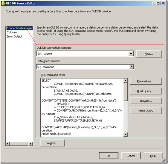
image

SQL Command Code:

SELECT 
    CONVERT(VARCHAR(50),@@SERVERNAME) AS ServerName,
    j.[job_id] AS JobId,
    CONVERT(VARCHAR(50),j.NAME) AS JobName,
    CONVERT(DATETIME,CONVERT(VARCHAR(8),jh.[run_date]) 
    + SPACE(1) 
    + STUFF(STUFF(RIGHT(REPLICATE('0',6) 
    + CONVERT(VARCHAR(6),run_time),6),3,0,':'),6,0,':')) AS rundate,
    Run_Status.descr AS jobstatus,
    STUFF(STUFF(RIGHT(REPLICATE('0',6) 
    + CONVERT(VARCHAR(6),Run_Duration),6),3,0,':'),6,0,':') AS duration
FROM msdb..[sysjobs] j
INNER JOIN msdb..[sysjobschedules] jsch
    ON j.[job_id] = jsch.[job_id]
INNER JOIN msdb..[sysschedules] sch
    ON jsch.[schedule_id] = sch.[schedule_id]
INNER JOIN msdb..[sysjobhistory] jh
    ON jh.[job_id] = j.[job_id]
INNER JOIN(
    SELECT 0 AS run_status ,'Failed' AS descr UNION ALL
    SELECT 1,'Succeeded' UNION ALL
    SELECT 2,'Retry' UNION ALL
    SELECT 3,'Canceled' UNION ALL
    SELECT 4,'In progress'
) AS Run_Status
    ON jh.[run_status] = Run_Status.[run_status]
WHERE
    j.NAME NOT LIKE 'Tivoli%' --tivoli backups
    AND j.[enabled] = 1
    AND sch.[enabled] = 1
    AND jh.[step_name] = '(Job outcome)'
    AND CONVERT(DATETIME,CONVERT(VARCHAR(8),jh.[run_date]) 
        + SPACE(1) 
        + STUFF(STUFF(RIGHT(REPLICATE('0',6) 
        + CONVERT(VARCHAR(6),run_time),6),3,0,':'),6,0,':')) 
        BETWEEN DATEADD(DAY,DATEDIFF(DAY,0,GETDATE()),0)
            AND DATEADD(DAY,DATEDIFF(DAY,0,GETDATE())+1,0)

Make sure to click the columns tab so SSIS can automatically set your columns for you.

Now let’s configure the destination.  The destination is actually quite simple.  We have to open the properties and choose our  SQLMngt_DW source and the JobHistory table, as shown below.  Make sure to select the mappings tab to verify all the columns are aligning properly.  You may see the JobHistoryId column is set to ignore, which is fine because this is an identity column and we do not want to insert directly into it.

image

Now we get to do the fun part :-), which is setting up the dynamic connection string via the connectionstring variable.  Right-click the dyn_source connection string and click properties.  Once the properties display, you can click the ellipses next to expressions and choose connectionstring.  Click the ellipses in the expression textbox to open the expression editor and paste the following expression:

"Data Source=" + @[User::ConnectionString] + ";Initial Catalog=msdb
;Provider=SQLNCLI10.1;Integrated Security=SSPI"
 
Note: I am using Integrated security. If your connection string is use SQL Authentication, you will need to supply username and password in the connection string.

image

Believe it or not, that is it!!!!   Click on the play sign at the top of the SSIS application to run the package.  We should see all tasks light up green, unless something is not configured correctly, in which case you will see red. 

image

Our last step is to validate our package did what it is supposed to do.  We can validate this by querying our job table.
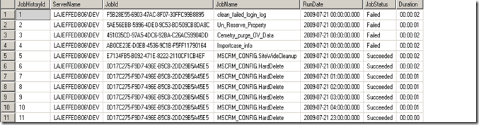
image

There you have it.  You now have a very flexible and scalable method to collect data from one or more sources.  The SSIS method really beats having to manage a command line solution or having to manage/deploy stored procedures to each server.  Configuring the SSIS package is not that tedious and can be done fairly quickly.  It actually takes a lot longer to describe how to do this, than actually do it.  Once you get use to using SSIS, this process should only take you 10-15 minutes to setup and configure.   I hope that you have learned something new and I know this will help some of you out there.  I know this post may seem overwhelming for those of you have not really had the opportunity to dive into SSIS yet, so I have provided a link, where you can download the project.  Please be aware that I am using SQL 2008 and BIDS 2008, so my package will not work with BIDS 2005, as the package structure changed in BIDS 2008.

Download the project files: http://cid-6f041c9a994564d8.skydrive.live.com/self.aspx/.Public/SSIS%7C_Data%7C_Collection/SSIS%7C_DataCollection.zip

Happy coding!!

Wednesday, June 24, 2009

Are valid search arguments still relevant?

I have seen a lot queries written in forums and from differing developers over the past few years and have noticed an increasing trend in “sloppy” code. Most of the “sloppy’” code that I am referring to has either an invalid search argument, or a function in the predicate. It seems developers these days are in such a rush to get code out they forget the principal mechanics of a properly tunned query. A lot of times a developer will put whatever in the predicate without knowing the performance implications. So how exactly do these type of queries affect performance? The short answer is the optimizer typically has to use an index/table scan to satisfy the query because the filters are not adequate to seek the row. In this post, I will be primarily focusing on invalid search arguments (non SARGable queries).

We will start of by defining what valid search arguments are. Essentially you should have an inclusive operator to seek an index. So what the heck is an inclusive operator? Inclusive operators are =, BETWEEN, >, >=, <=, <, and like (begins with only). Now that we have our valid search arguments, we know that our query predicate should include one of these operators; otherwise, an index seek will be unlikely. You will notice that the list of available operators does not include: IS NULL, IS NOT NULL, <>, and like (contains). Does this mean that these operators are incapable of using a seek? No, it does not. It should be known that the optimizer may not be able to generate accurate cardinality estimates for the “not equal to” operator. What I want to dig into is the implications of using invalid search arguments and I will be focus on the “<>” operator.

Let’s start by creating and populating a sample table.

USE [tempdb]
GO
 
IF OBJECT_ID('dbo.TestData') IS NOT NULL
BEGIN
    DROP TABLE dbo.[TestData];
END
GO
 
SELECT TOP 100000 
    RowNum   = IDENTITY(INT,1,1),
    SomeID   = ABS(CHECKSUM(NEWID()))%2500+1, 
    SomeCode = CHAR(ABS(CHECKSUM(NEWID()))%26+65)
             + CHAR(ABS(CHECKSUM(NEWID()))%26+65)
INTO dbo.TestData
FROM Master.dbo.SysColumns t1,
    Master.dbo.SysColumns t2 
GO
        
ALTER TABLE dbo.TestData
ADD PRIMARY KEY CLUSTERED (RowNum);
GO
 
CREATE INDEX IXC_TestData_Cover1 ON dbo.TestData(SomeId) ;
GO
CREATE INDEX IXC_TestData_Cover2 ON dbo.TestData(somecode) ;
GO

Now that we have our table, lets start by running a simple query using “not equal to.”

DBCC DROPCLEANBUFFERS
DBCC FREEPROCCACHE
 
SELECT
    rownum,
    someid, 
    [SomeCode]
FROM dbo.[TestData] t1
WHERE
    t1.[SomeId] <> 0

Here is the query plan and the IO/TIME stats

image

SQL Server parse and compile time:

   CPU time = 0 ms, elapsed time = 0 ms.

Table 'TestData'. Scan count 1, logical reads 238, physical reads 1, read-ahead reads 146, lob logical reads 0, lob physical reads 0, lob read-ahead reads 0.


 SQL Server Execution Times:

   CPU time = 47 ms,  elapsed time = 1477 ms.


 SQL Server Execution Times:

   CPU time = 0 ms,  elapsed time = 0 ms.

As you can see, the query performed like we thought it would by scanning the index to satisfy the query, but what happens when we cover the query with our index? The answer may be quite surprising. To test this we need to reduce the number of columns in the select list.

Here is the new query: Note: we can leave rownum in the select list because this column is part of the clustering key, which is included in non clustered indexes.

SET NOCOUNT ON;
GO
 
DBCC DROPCLEANBUFFERS
DBCC FREEPROCCACHE
 
SET STATISTICS IO ON;
SET STATISTICS TIME ON;
 
SELECT
    rownum,
    someId
FROM dbo.[TestData] t1
WHERE
    t1.[SomeId] <> 0
 
SET STATISTICS IO OFF;
SET STATISTICS TIME OFF;

Here is the query plan and the IO/TIME stats

image

SQL Server parse and compile time: CPU time = 0 ms, elapsed time = 0 ms. Table 'TestData'. Scan count 2, logical reads 179, physical reads 1, read-ahead reads 153, lob logical reads 0, lob physical reads 0, lob read-ahead reads 0.

SQL Server Execution Times: CPU time = 94 ms, elapsed time = 1207 ms.

SQL Server Execution Times: CPU time = 0 ms, elapsed time = 0 ms.

The results are pretty interesting. We actually get an index seek because of the covering index, but the IO and CPU Time actually increased. You are probably screaming at the screen saying,” HOLD ON BUDDY YOU JUST SAID THAT <> IS NOT A VALID SEARCH ARGUMENT!!!” and you would be right. The answer is actually quite simple…. the “not equal to” operator did NOT seek the row. If you mouse over the index seek show plan operator you will see that the seek predicate actually gets transformed into a > and <. So this is where myself and other SQL Server enthusiasts debate . This begs the question that if the optimizer can change the “not equal to” operator into a ranged search… does this make “not equal to” a valid search argument? I leave this up to you to decide, I however say no. In my opinion, the < and > are valid search operators, not the "<>". I cannot find any documentation on how/when the predicate transformation actually occurs. The main question I have is, can we definitively say that the optimizer will ALWAYS transform the predicate. If the answer is yes, then we can say it is a valid search argument, but until then I have to say no. I will most definitely agree that the optimizer is usually pretty smart in using the index to search inequalities. Here is a screenshot of the index show plan operator.

image

Now let’s do what I like to do and rewrite inequalities to be valid SARG.

SET NOCOUNT ON;
GO
 
DBCC DROPCLEANBUFFERS
DBCC FREEPROCCACHE
 
SET STATISTICS IO ON;
SET STATISTICS TIME ON;
 
SELECT
    rownum,
    someId
FROM dbo.[TestData] t1
WHERE
    t1.[SomeId] < 0 OR t1.[SomeID] > 0
 
SET STATISTICS IO OFF;
SET STATISTICS TIME OFF;

The query plan and IO/Time Stats:

image

SQL Server parse and compile time: CPU time = 0 ms, elapsed time = 0 ms. Table 'TestData'. Scan count 2, logical reads 179, physical reads 1, read-ahead reads 153, lob logical reads 0, lob physical reads 0, lob read-ahead reads 0.

SQL Server Execution Times: CPU time = 94 ms, elapsed time = 1207 ms.

SQL Server Execution Times: CPU time = 0 ms, elapsed time = 0 ms.

So what’s the verdict? Well in this case the optimizer choose the exact same plan with the exact same IO/CPU time.  So where does that leave us?  I invite each of you to decide for yourselves, but my opinion is to stick with best practices and with valid search arguments.  While these queries are theoretically the same, I believe a predicate should be as SARG friendly as possible. In doing so the developer can ensure the optimizer is able to make the best decision possible. The questions on the table are, How consistent is the optimizer in transforming the query, especially if the optimizer cannot accurately measure cardinality and are valid search arguments still relevant? I cant answer the first question now, perhaps I can come up with an example, but this is a question maybe more appropriate for the query optimization team. I answer yes to SARG relevance. Valid search arguments give the optimizer better cardinality estimates and is a more inclusive search, which usually translates into better and more consistent performance. With that said, the optimizer is able to handle many invalid search argument variants and successfully transform those queries into something useful, but do we really want to rely on the optimizer to  “automagically” fix our code?

Links:

Tuesday, June 16, 2009

Superfluous columns…. more than a bad habit?

Are using superfluous columns, in a SELECT list, bad? Sure they are and for a multitude of reasons. The better question is, why do developers still use superfluous columns, knowing that they should not?  I believe developers get tunnel vision and forget to look at the big picture,  perhaps it is laziness, or perhaps the developer does not care because company policy is to fix performance problems with bigger hardware, which is common these days. For whatever the reason, tunnel vision and laziness usually lead to rapidly developed, non-performant code. Developers often forget the overall impact bad code can have on a system, no matter how simple.  The impact depends on varying factors including: access frequency, bytes returned, query performance etc... I am going to explore why superfluous columns are not a best practice.

Let’s get started by creating a sample table with a million rows.

USE [tempdb]
GO
 
IF OBJECT_ID('test..t') IS NOT NULL
DROP TABLE t
GO
 
SELECT TOP 1000000 --<<<LOOK! CHANGE THIS NUMBER TO CHANGE THE NUMBER OF ROWS!

        RowNum   = IDENTITY(INT,1,1),
        SomeID   = ABS(CHECKSUM(NEWID()))%2500+1, --<<<LOOK! CHANGE THIS NUMBER TO 1/400th THE ROW COUNT
        SomeCode = CHAR(ABS(CHECKSUM(NEWID()))%26+65)
                 + CHAR(ABS(CHECKSUM(NEWID()))%26+65),
        SomeCode2 = CHAR(ABS(CHECKSUM(NEWID()))%26+65)
                    + CHAR(ABS(CHECKSUM(NEWID()))%26+65)
                    + CHAR(ABS(CHECKSUM(NEWID()))%26+65)
                    + CHAR(ABS(CHECKSUM(NEWID()))%26+65),
        SomeCode3 = CHAR(ABS(CHECKSUM(NEWID()))%26+65)
                    + CHAR(ABS(CHECKSUM(NEWID()))%26+65)
                    + CHAR(ABS(CHECKSUM(NEWID()))%26+65)
                    + CHAR(ABS(CHECKSUM(NEWID()))%26+65)
   INTO dbo.t
   FROM Master.dbo.SysColumns t1,
        Master.dbo.SysColumns t2 
 
--===== Add the index to support both types of queries
CREATE INDEX IXC_TestData_Cover1 ON dbo.t(SomeID,SomeCode)
GO

Now that we have our table and test data, let’s run a simple query using select * and another select statement that uses fewer columns.  You should enable client statistics to view the bytes returned to the client.

Note: You can enable this via the toolbar, shown below, or by clicking the option from the query menu.

image 

First run the query with superfluous columns ( Make sure you enable client statistics)

SELECT *
FROM dbo.t
WHERE
    someid < 500
GO

Now let’s run the query with fewer columns:

SELECT 
    RowNum,
    SomeID,
    SomeCode
FROM dbo.t
WHERE
    someid < 500
GO

The client statistics between the two runs should look similar to the screenshot below.  You will notice that the bytes received from the server has drastically decreased, for the query with fewer columns in the SELECT list. The bytes sent from client is the number of bytes that make up the query text, which is irrelevant to our tests.

image

The value of interest is Bytes received from server.  This represents the number of bytes to the client, from the server.   In our case, the bytes dropped from 1024209 to 551576.  To put the number of bytes reduced into perspective, lets crunch the numbers.  We know that the superfluous query used 1024209 bytes. We can transform this into the number of  MBs returned. We are going to base these numbers on a concurrent user load of 500 users. Our calculation becomes. ((Number of bytes * number of concurrent users) / 1024.0) / 1024.0.  The result of this calculation is shown below.


Bytes

KB

MB

Superfluous Columns

512104500

500102.1

488.381

Non-Superfluous Columns

275788000

269324.2

263.012

As you can see, the number of bytes returned by the superfluous query is over 200 MB larger. This may not seem like much, but this is only one query and imagine if you have a 1000 concurrent users.  The superfluous column query would return approximately 500MB more data. This means the superfluous query would return nearly 1GB of data… now that is huge!

By selecting the columns we need, we are able to reduce the amount of data the web server has to process, which can lead to faster load times, less consumed resources, and a better end user experience.

So, your probably sold on the idea that superfluous columns are bad, but I have one more point to make.  Not only does the query return more bytes, but superfluous columns can affect the optimizer’s ability to use a covering index, even in a derived table/CTE.

Using the same sample, with a slight modification.

Superfluous query:

SELECT *
FROM dbo.t
WHERE
    someid = 100
GO

Below is the query plan.  What you see is that our index was able to be used; however, the index does not contain all the columns in our SELECT list, thus the optimizer has to go back to the HEAP to get the remaining column data.

Note: depending on the indexes in place the RID look could be replaced by a Key Lookup, if a clustered index exists.

image

Here is the non-superfluous column query:

SELECT 
    SomeID,
    SomeCode
FROM dbo.t
WHERE
    someid = 100
GO

These are the results from the query with non-superfluous columns:

image

You can test the same results with a CTE:

--this yeilds an index RID lookup
;WITH cte
AS
(
    SELECT 
        [RowNum]
        [SomeId],
        [SomeCode],
        [SomeCode2],
        [SomeCode3]
    FROM t
    WHERE 
        [SomeId] = 100
)
SELECT 
    [SomeId],
    [SomeCode]
FROM cte
 
--this yields an index seek via covering index
;WITH cte
AS
(
    SELECT 
        [SomeId],
        [SomeCode]
    FROM t
    WHERE 
        [SomeId] = 100
)
SELECT 
    [SomeId],
    [SomeCode]
FROM cte

Results:

Superfluous columns:

image

Non-superfluous columns:

image

So there you have it. Selecting more columns than you need, not only affects application performance, it affects the number of bytes returned to the client. All of these factors can  directly affect the user’s experience, which should be very important to developer/DBA staff.  Additionally, superfluous columns can cause bookmark lookups, which will degrade database performance.