Monday, August 31, 2009

Pivoting Data Using SQL 2005 (Part 3)

If you have been following this series, I have been focusing on many different aspects of dynamic pivoting using SQL 2005. In the first part of this series,http://jahaines.blogspot.com/2009/08/pivoting-data-using-sql-2005-part-1.html, I focused on creating a static pivot query. In the second part of this series, http://jahaines.blogspot.com/2009/08/pivoting-data-using-sql-2005-part-2.html,I focused on creating a dynamic pivot, where the pivot values were unknown. We are now going to ramp up this series with a completely dynamic pivot. In this series, will will pivot data where the columns are stored as rows in a table and the values are not known.

In this example, we will be looking at employee sales. Let’s start by creating and populating our sample tables.

SET NOCOUNT ON
GO
 
IF OBJECT_ID('tempdb..#Pivot_Columns') IS NOT NULL
BEGIN
    DROP TABLE #Pivot_Columns;
END
GO
 
CREATE TABLE #Pivot_Columns(
ColId INT PRIMARY KEY,
TableName VARCHAR(25),
ColName VARCHAR(25)
);
GO
 
INSERT INTO #Pivot_Columns VALUES (1,'#Sales','YearMonth');
INSERT INTO #Pivot_Columns VALUES (2,'#Sales','SalesAmt');
 
IF OBJECT_ID('tempdb..#EmpSales') IS NOT NULL
BEGIN
    DROP TABLE #EmpSales;
END
GO
 
CREATE TABLE #EmpSales(
EmpSalesId INT IDENTITY(1,1) PRIMARY KEY,
EmpId INT,
SalesId INT,
ColId INT,
ColTxt VARCHAR(50)
);
GO
 
INSERT INTO #EmpSales VALUES (1,1,1,'2008-08');
INSERT INTO #EmpSales VALUES (1,1,2,'10000');
INSERT INTO #EmpSales VALUES (2,3,1,'2008-07');
INSERT INTO #EmpSales VALUES (2,3,2,'8500.25');
INSERT INTO #EmpSales VALUES (3,4,1,'2008-08');
INSERT INTO #EmpSales VALUES (3,4,2,'5999.99');

Now we have our table, let’s have a look at an example.

DECLARE @sql NVARCHAR(MAX),
        @Pivot_Cols VARCHAR(MAX)
    
--The code below reads through all the data in the table and
--builds a distinct column list.
SELECT 
    @Pivot_Cols = COALESCE(@Pivot_Cols + ',','') + QUOTENAME(ColName)
FROM #Pivot_Columns
GROUP BY QUOTENAME([ColName])
ORDER BY QUOTENAME(ColName) ASC
 
SELECT @sql = N'
SELECT 
    EmpId,' + @Pivot_Cols + '
FROM(
    SELECT e.EmpId,    e.ColTxt,pc.ColName
    FROM #EmpSales e
    INNER JOIN #Pivot_Columns pc ON e.ColId = pc.ColId
) AS dataToPivotTable
PIVOT(
    MAX(ColTxt) --Aggregate Function
    FOR [ColName]-- Column To Pivot
    IN (' + @Pivot_Cols + ') --Values to Pivot
) AS whatToPivotOnTable;'
 
--PRINT @sql
EXEC sp_executesql @sql
GO

Results:

image

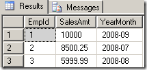
As you can see from the screenshot above, we have successfully pivoting the rows of data into columns. Is this all that there is to dynamic pivoting?…..not quite. If you look closely at the example above you will notice that we are using the MAX aggregate to get the maximum of each column. This is fine if you expect a single set of rows, but what do you think will happen when an employee has more than one set of rows? The short answer is the data would be rendered invalid. The data may become invalid because the maximum YearMonth value, may be from a different month than the maximum SalesAmt value. To demonstrate this behavior, we will add a new set of rows into our table.

INSERT INTO #EmpSales VALUES (1,2,1,'2008-09');
INSERT INTO #EmpSales VALUES (1,2,2,'1');

Now execute the same query and your results should look like the screenshot below. The sales amount column has a maximum value of 10,000 and the YearMonth is 2008-09. If you look carefully at the data we inserted, the SalesAmt value should be 1, for 2008-09, not 10,000.

image

So how do we resolve this issue? Let’s press on. We are going to modify our query a bit.

DECLARE @sql NVARCHAR(MAX),
        @Pivot_Cols VARCHAR(MAX)
    
--The code below reads through all the data in the table and
--builds a distinct column list.
SELECT 
    @Pivot_Cols = COALESCE(@Pivot_Cols + ',','') + QUOTENAME(e.ColTxt)
FROM #EmpSales e
INNER JOIN [#Pivot_Columns] pc
    ON e.[ColId] = pc.[ColId]
WHERE pc.[ColName] = 'YearMonth'
GROUP BY QUOTENAME(e.ColTxt)
ORDER BY QUOTENAME(e.ColTxt)
 
SELECT @sql = N'
SELECT 
    EmpId,' + @Pivot_Cols + '
FROM(
    SELECT 
        e.EmpId,
        e.ColTxt as MonthYear,
        CONVERT(NUMERIC(9,2),e2.[ColTxt]) AS [ColTxt]
     FROM #EmpSales e INNER JOIN #EmpSales e2 ON e.EmpId = e2.EmpId AND e.SalesId = e2.SalesId 
     INNER JOIN #Pivot_Columns pc ON pc.ColID = e.[ColId]
     INNER JOIN #Pivot_Columns pc2 ON pc2.ColId = e2.[ColId]
     WHERE pc.ColName = ''YearMonth'' AND pc2.ColName = ''SalesAmt''
) AS dataToPivotTable
PIVOT(
    SUM([ColTxt]) --Aggregate Function
    FOR [MonthYear]-- Column To Pivot
    IN (' + @Pivot_Cols + ') --Values to Pivot
) AS whatToPivotOnTable;'
 
PRINT @sql
EXEC sp_executesql @sql
GO

The code is very similar in most respects, but the biggest difference is I am not pivoting on ColName. Instead, I am going back to the methods we learned in part 2 of this series. The key to dynamically pivoting data is to know your data. Depending on what you are trying to pivot, you may need to aggregate data or simply use the MAX pivot. In this case, we need to use a more powerful pivot statement. In the variable assignment portion of the modifed code, I am strictly querying #EmpSales table, making sure to filter for column “YearMonth.” Within the Pivot code, I select the needed data by using a self referencing join. We need a self join because our next step is to create a row of data that contains the SalesAmt for each EmpId’s salesId. Once we have this information we can use the pivot operator to perform the aggregation.

Results:

image

How about them apples? As you can see, the new pivot reflects the correct totals for each month. We can also create a version of this code that works with prior versions of SQL Server.

DECLARE @Pivot_Cols VARCHAR(MAX)
DECLARE @sql NVARCHAR(MAX)
 
SELECT 
    @Pivot_Cols = COALESCE(@Pivot_Cols + ',','') 
    + N'SUM(CONVERT(NUMERIC(9,2),CASE WHEN pc.[ColName] = ''YearMonth'' AND e.ColTxt =' 
    + QUOTENAME(e.ColTxt,'''') + ' THEN ' + ' e2.[ColTxt] ELSE NULL END)) AS ' 
    + QUOTENAME(e.ColTxt,'''') + CHAR(13)    
FROM #EmpSales e
WHERE e.ColId = 1
GROUP BY e.ColTxt
ORDER BY e.ColTxt
 
SET @sql = N'SELECT e.EmpId,' + CHAR(13)
      + @Pivot_Cols + CHAR(13) 
      + 'FROM #EmpSales e INNER JOIN #EmpSales e2 ON e.EmpId = e2.EmpId AND e.SalesId = e2.SalesId' + CHAR(13) 
      + 'INNER JOIN #Pivot_Columns pc ON pc.ColID = e.[ColId]' + CHAR(13)
      + 'INNER JOIN #Pivot_Columns pc2 ON pc2.ColId = e2.[ColId]' + CHAR(13)
      + 'WHERE pc.ColName = ''YearMonth'' AND pc2.ColName = ''SalesAmt''' + CHAR(13)
      + 'GROUP BY e.[EmpId]'
      
PRINT @sql
EXEC sp_executesql @sql

So there you have it. A completely dynamic method to pivot data. So what have we learned over these last few posts………….. well I hope that you have learned something :-). I hope that you learned pivoting data in SQL Server can be very simple. Pivoting data can sometimes become a little hairy, but is still a powerful and somewhat simplistic solution to implement. <step on soapbox> Hopefully, Microsoft will give us a pivot operator that is somewhat flexible and dynamic. A native dynamic pivot operator allows for more scalable code and reduced SQL injection risk.; however, I really doubt that we will get any dynamic pivot operator, in the near future</step off soapbox>. Anyway, I hope that you have enjoyed reading this series and that you can use this in your environment.

Until next time… happy coding.

Thursday, August 20, 2009

Pivoting Data Using SQL 2005 (Part 2)

This is part two of a three part series focusing on pivoting data, using SQL Server 2005. In part one of the series, I focused on creating a static pivot using the pivot operator, http://jahaines.blogspot.com/2009/08/pivoting-data-using-sql-2005-part-1.html. In this post, I will be focusing on creating a dynamic pivot where the pivot values are not known.  I choose to use a differing sample of data than the first part of this series.  The code in the first part became too complex for simple demonstration.  The code became complex due to my having to calculate column quarters values.  I have attached the dynamic pivot solution, for the part one data, which can be found at the end of this article.  Let’s get started with our new table and data.

Table/Data

SET NOCOUNT ON
GO
 
IF OBJECT_ID('tempdb..#Orders') IS NOT NULL
BEGIN
    DROP TABLE #Orders;
END
GO
 
CREATE TABLE #Orders(
OrderId INT IDENTITY(1,1) PRIMARY KEY,
CustId INT NOT NULL,
ProductDescr VARCHAR(50),
Sales_Dt DATETIME,
Sales_Amt NUMERIC(9,2)
);
GO
 
INSERT INTO #Orders VALUES (1,'Product1','2008-01-01',0.99);
INSERT INTO #Orders VALUES (2,'Product1','2008-04-01',1.99);
INSERT INTO #Orders VALUES (1,'Product3','2009-01-01',100.25);
INSERT INTO #Orders VALUES (1,'Product4','2009-02-01',999.99);
INSERT INTO #Orders VALUES (2,'Product2','2009-01-01',99.99);
INSERT INTO #Orders VALUES (2,'Product1','2009-01-03',107.20);
INSERT INTO #Orders VALUES (3,'Product4','2009-01-03',459.36);
INSERT INTO #Orders VALUES (3,'Product3','2009-05-01',19.99);
INSERT INTO #Orders VALUES (3,'Product5','2009-06-01',29.99);
GO

Now that we have our table, let’s start coding.  The driving force behind the code below is the variable assignment.  We build the column/value list dynamically by creating a process that appends distinct values to an existing string.  Once we have the column list, we just have to create the same query that we created in part one of this series and append the variables.  I created two variables to house the columns.  The variable @Cols is used to create our select list which ultimately is the value wrapped in the coalesce function.  For example, COALESCE([Product1],0) AS [Product1],COALESCE([Product2],0) AS [Product2]…..  The Second variable @Pivot_Cols is used to store the column metadata, in the format [Product1],[Product2],…  There are many different ways to accomplish variable assignment, but I tend to like the COALESCE method.  I will show you another method later on.

DECLARE @sql NVARCHAR(MAX),
        @cols VARCHAR(MAX),
        @Pivot_Cols VARCHAR(MAX)
    
--The code below reads through all the data in the table and
--builds a distinct column list.
SELECT 
    @cols = COALESCE(@cols + ',','') 
        + 'COALESCE(' + QUOTENAME(ProductDescr) + ',0) AS ' + QUOTENAME(ProductDescr),
    @Pivot_Cols = COALESCE(@Pivot_Cols + ',','') + QUOTENAME(ProductDescr)
FROM #Orders
GROUP BY QUOTENAME(ProductDescr)
ORDER BY QUOTENAME(ProductDescr) ASC
 
SELECT @sql = N'
SELECT 
    CustId,' + @Cols + '
FROM(
    SELECT 
        CustId,
        ProductDescr,
        Sales_Amt    
    FROM #Orders
    WHERE
        Sales_Dt >= ''2008-01-01''
        AND Sales_Dt < ''2010-01-01''
) AS dataToPivotTable
PIVOT(
    SUM(Sales_Amt) --Aggregate Function
    FOR [ProductDescr]-- Column To Pivot
    IN (' + @Pivot_Cols + ') --Values to Pivot
) AS whatToPivotOnTable;'
 
PRINT @sql
EXEC sp_executesql @sql

Note: I hard coded the date filters, but I advise you too use supply the date parameters using sp_executesql, as this will allow you to help parameterize the query.

Results:

image

We can also expand on our SQL 2000 solution, as shown below.

DECLARE @Cols VARCHAR(MAX)
DECLARE @sql NVARCHAR(MAX)
 
SELECT @cols = 
    MAX(COALESCE(@cols + ',','') 
    + N'SUM(CASE WHEN ProductDescr = '
    + QUOTENAME(ProductDescr,'''') + ' THEN Sales_Amt ELSE 0 END) AS ' 
    + QUOTENAME(ProductDescr))
FROM #Orders
GROUP BY QUOTENAME(ProductDescr)
ORDER BY QUOTENAME(ProductDescr) ASC
 
SET @sql = N'SELECT CustId,' + CHAR(13)
      + @Cols + CHAR(13) 
      + 'FROM #Orders' + CHAR(13) 
      + 'WHERE Sales_Dt >= ''2008-01-01'' AND Sales_Dt < ''2010-01-01'' ' + CHAR(13) 
      + 'GROUP BY CustId'
 
PRINT @sql
EXEC sp_executesql @sql

As promised, here is another method to solve variable assignment.

SELECT @cols =  
    STUFF((
        SELECT DISTINCT TOP 100 PERCENT 
            ',' + N'SUM(CASE WHEN ProductDescr = '
            + QUOTENAME(ProductDescr,'''') + ' THEN Sales_Amt ELSE 0 END) AS ' 
            + QUOTENAME(ProductDescr)
        FROM #Orders
        ORDER BY 
            ',' + N'SUM(CASE WHEN ProductDescr = '
            + QUOTENAME(ProductDescr,'''') + ' THEN Sales_Amt ELSE 0 END) AS ' 
            + QUOTENAME(ProductDescr) ASC
        FOR XML PATH (''))
        ,1,1,'')

As you can see, the dynamic pivot is fairly easy to implement.  It is much easier to dynamically pivot data when you do not have to calculate your column values. If you are wondering why I did not show solve the example from the last post (Maybe because you did not read the beginning of this post :-) , I choose not to post this solution because it is a little more complex because you have to calculate the column value; however, I will be attaching the solution via my sky drive.   I hope that you are still awake and ready for more pivoting fun because in part three of this series I am taking dynamic pivoting to the extreme.  In part 3, I will be making every single aspect of the pivot dynamic, including using column names that are stored as rows in a table.

Until next time, happy coding.

Dynamic solution – part1 data: http://cid-6f041c9a994564d8.skydrive.live.com/self.aspx/.Public/Dynamic%7C_Pivot/DyamicPivot.sql

Sunday, August 16, 2009

Pivoting Data Using SQL 2005 (Part 1)

SQL Server 2005 introduced a new operator that makes pivoting data really easy.  For those of you who may be unfamiliar with the term pivot, pivoting is the process of transforming row values into columns, using an aggregate function to summarize data.  The biggest problem with the pivot operator is that the values have to be known, which severely limits the flexibility of the pivot. Hopefully, in future versions Microsoft will give us a more dynamic Pivot operator. In the interim, the only way to dynamically pivot data is to use dynamic SQL, which I will address in part 2 of this series.  For now let’s focus a on creating a simple Pivot query.  I will start by creating a sample table.

IF OBJECT_ID('tempdb..#Sales') IS NOT NULL
BEGIN
    DROP TABLE #Sales;
END
GO
 
CREATE TABLE #Sales(
Sales_Id INT IDENTITY(1,1) PRIMARY KEY,
Emp_Id INT,
Sales_Dt DATETIME,
Sales_Amt NUMERIC(9,2)
);
GO
 
INSERT INTO #Sales VALUES (1,'2009-01-01',100.25);
INSERT INTO #Sales VALUES (1,'2009-02-01',999.99);
INSERT INTO #Sales VALUES (1,'2009-03-01',499.99);
INSERT INTO #Sales VALUES (1,'2009-04-15',654.99);
INSERT INTO #Sales VALUES (1,'2009-07-06',197.99);
INSERT INTO #Sales VALUES (2,'2009-01-01',99.99);
INSERT INTO #Sales VALUES (2,'2009-01-03',107.20);
INSERT INTO #Sales VALUES (3,'2009-01-03',459.36);
INSERT INTO #Sales VALUES (3,'2009-05-01',19.99);
INSERT INTO #Sales VALUES (3,'2009-06-01',29.99);
INSERT INTO #Sales VALUES (3,'2009-07-01',1250.98);
INSERT INTO #Sales VALUES (3,'2009-04-01',488.23);
INSERT INTO #Sales VALUES (3,'2009-02-28',1999.99);
GO

Now that we have our table, we can create our pivot query.  The Pivot operator has three crucial components, the aggregate function, the column to pivot, and the row values to aggregate into columns.  In the example below, we are using the aggregate function SUM, pivoting the column Qtr, (which is expressed as the quarter datapart of the Sales_Dt), and aggregating the Sales_Amt for sales_dates that fall within Quarters “1,2,3,4”. 

Note: I limited the data to the current year.  If multiple years are returned the values may not aggregate correctly because quarters will overlap between years.  We will address this problem in part 2, of this series by appending the year to the pivot values.

SELECT 
    Emp_Id,
    COALESCE([1],0) AS [Q1],
    COALESCE([2],0) AS [Q2],
    COALESCE([3],0) AS [Q3],
    COALESCE([4],0) AS [Q4]
FROM(
    SELECT 
        Emp_id,
        DATEPART(QUARTER,Sales_Dt) AS [Qtr],
        Sales_Amt    
    FROM #Sales
    WHERE
        Sales_Dt >= '2009-01-01'
        AND Sales_Dt < '2010-01-01'
) AS dataToPivotTable
PIVOT(
    SUM(Sales_Amt) --Aggregate Function
    FOR [Qtr]-- Column To Pivot
    IN ([1],[2],[3],[4]) --Qtr Values to Pivot
) AS whatToPivotOnTable;

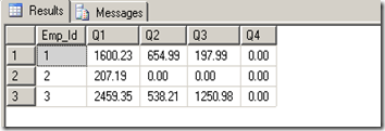
image

I would like to take a minute to describe what the pivot operator is doing, in the background.  I believe the easiest way to understand what is occurring  is to break apart each key component.  For example, the pivot column, or the column used in the FOR clause,  is the column that you want to group by, the the aggregate function aggregates and summarizes data  (No surprises there :-) , and the row values used in the IN clause are used to create a case expression. Under the hood the pivot operator can be expressed as:

 
SELECT 
Aggregate_Function(CASE WHEN MyCol = MyValue1 THEN MyCol ELSE NULL END),
Aggregate_Function(CASE WHEN MyCol = MyValue2 THEN MyCol ELSE NULL END),
...
FROM MyTable GROUP BY GroupByColumn

You can look at the execution plan of the Pivot query to validate that this is occurs, in the stream aggregate show plan operator.  The same construct can be used to create a pivot or a  “Cross-Tab” query, in prior versions on SQL Server.  We can evaluate the very same pivot statement, as shown below.

SELECT 
    [Emp_Id],
    SUM(CASE WHEN DATEPART(QUARTER,Sales_Dt) = 1 THEN Sales_Amt ELSE 0 END) AS [Q1],
    SUM(CASE WHEN DATEPART(QUARTER,Sales_Dt) = 2 THEN Sales_Amt ELSE 0 END) AS [Q2],
    SUM(CASE WHEN DATEPART(QUARTER,Sales_Dt) = 3 THEN Sales_Amt ELSE 0 END) AS [Q3],
    SUM(CASE WHEN DATEPART(QUARTER,Sales_Dt) = 4 THEN Sales_Amt ELSE 0 END) AS [Q4]
FROM #Sales
WHERE
    Sales_Dt >= '2009-01-01'
    AND Sales_Dt < '2010-01-01'
GROUP BY [Emp_Id];

There you have it.  A simplistic method to pivot rows of data into columns.  In part 2 of this series, I will focus on creating a dynamic pivot statement, where the columns and values are unknown.

Happy coding.

Friday, August 7, 2009

Are all covering indexes created equal?

I have been getting a lot of questions regarding indexes over the past few weeks, so I thought I would make another post about indexes. In this post, I will be focusing on covering indexes.  A covering index is an index that covers all the columns for a given query.  A covering index can be created by either, adding the columns to the index key, or by adding the columns to the include clause of the create index statement. I will focus on the key differences between adding columns to the index key and adding columns to the INCLUDE clause.  I will look at the differences in size, statistics, and the execution plan.

Let’s get started by creating our test table.

USE [tempdb]
GO
 
SET NOCOUNT ON;
GO
 
IF EXISTS(SELECT 1 FROM sys.tables WHERE NAME = 'TestData')
BEGIN
    DROP TABLE dbo.[TestData];
END
GO
 
CREATE TABLE dbo.TestData(
RowNum INT PRIMARY KEY,
SomeId INT,
SomeCode INT
);
GO
 
INSERT INTO dbo.[TestData] (
    [RowNum],
    [SomeId],
    [SomeCode]
) 
SELECT TOP 1000000 
    ROW_NUMBER() OVER (ORDER BY t1.NAME) AS RowNum,
    ABS(CHECKSUM(NEWID()))%2500+1 AS SomeId, 
    CASE 
        WHEN ROW_NUMBER() OVER (ORDER BY t1.NAME) % 2 = 0
        THEN 1
    ELSE 0
    END AS SomeCode
FROM 
    Master.dbo.SysColumns t1,
    Master.dbo.SysColumns t2
GO

Now that we have our test table, I will create a covering index using the INCLUDE clause.

CREATE INDEX ncl_idx_TestData_Cover1 ON dbo.TestData(SomeID) INCLUDE(SomeCode);
GO

I will issue a simple query to select data from the table, using the new index.

SELECT 
    someid,
    somecode
FROM dbo.[TestData]
WHERE
    someid = 500 
    AND somecode = 1

The results of this query are inconsequential for our purposes, so I will not post them here; however, I will post the key attributes of the execution plan.

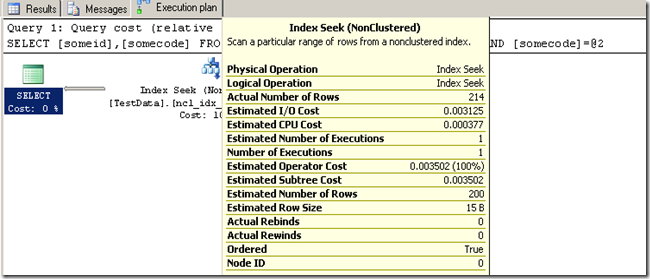
image 

The above screenshot shows that our covering index is used.  The primary thing to note here is deviation between the actual and the estimated number of rows. I will get into why these numbers deviate later in the post.

Let’s have a look at the space consumed by the index.  I will  issue a system stored procedure called sp_spaceused to obtain the space consumption details.

EXEC sp_spaceused 'dbo.Testdata' 

image

As you can see from the screenshot above, our index size is 18008 KB or  17.58 MB = 18008 / 1024. Now that we have our index size, let’s look at the statistics. I will be using the DBCC command show_statistics to display statistical information about our index.

DBCC show_statistics('dbo.Testdata','ncl_idx_TestData_Cover1')

image

The main thing to note here is that the column “SomeCode” is not available in the density vector.  The density vector is located in the second result set produced by DBCC show_statistics.  Essentially, density is the uniqueness of the column data. For example, the density of some id is .0004.  The density calculation can be expressed as 1/(#Distinct Values). In the case of “SomeId” the density can be calculated as 1/2500= .0004.  The “SomeId,RowNum” density is calculated as 1/1000000 = .000001. I know the number of distinct values is equal to the number of rows because “RowNum” is a unique column.  If you want to calculate density programmatically, you can use a group by clause and a little creativity.

Note: you can use differing columns in the group by clause to get their respective density.

SELECT 1./SUM(cnt)
FROM (
SELECT 1 AS cnt
FROM dbo.testdata
GROUP BY someid,RowNum
) AS a

The optimizer uses density to estimate cardinality (estimated number of rows) when building a query plan.  Obviously, the better the cardinality the better the query plan. 

A benefit of the INCLUDE clause is the ability to supersede index limitations, such as the key column limit of  16, the  index key size limitation (900 bytes), and even include columns with data types like VARCHAR(MAX), VARBINARY(MAX), TEXT, IMAGE etc..

Next, I will create the second covering index, which includes all columns in the index key. I will drop the original covering  index, so I can accurately measure the index size.

DROP INDEX ncl_idx_TestData_Cover1 ON dbo.[TestData];
GO
 
----===== Covering index that includes both columns in the index key
CREATE INDEX ncl_idx_TestData_Cover2 ON dbo.TestData(SomeID,SomeCode)
GO

Now let’s run the same select query again.

SELECT 
    someid,
    somecode
FROM dbo.[TestData]
WHERE
    someid = 500 
    AND somecode = 1

image

As you can see the estimated number of rows deviates much less, from the actual, than the first covering index.  The difference in cardinality estimates is pretty negligible for this sample, but in a real world scenario, the deviation can be much larger.

Let’s have a look at the space used.

Note: You can use the same code as before.

image

As shown above, the index size is larger, when columns are added to the index key.  The new covering index is 18024 KB or 18024 / 1024 = 17.60 MB.  This index is larger because the columns are stored at all levels of the index, whereas, the include clause stores the column values at the leaf level only.  So why would you add columns to the index key?  This answer brings us to the statistics maintained by the new index. 

Note: You can use the same code as before but change the name of the index to ncl_idx_TestData_Cover2.

image

If you had not noticed from the screen shot above, SQL Server is maintaining the density of the “SomeCode” column in relation to the “SomeId” column, which was not the case for covering index 1.  This is why the optimizer is able to more accurately estimate cardinality.  In this case, the density value is represented as .0002.  Adding columns to the index key allows the optimizer to make better cardinality estimates, which may translate into more optimal query plans.

So what is the verdict?  My findings indicate that all covering indexes are  not created equal.  Both types of covering index has its own strengths and weaknesses. The type you choose will depend on your query and your business requirements.  There are a lot of advantages to using both types of covering indexes.  You will have to weigh performance against manageability and choose which is best for your environment.

References:

Monday, August 3, 2009

TSQLChallenges.com

For those of you who like doing puzzles and have a desire to enhance your TSQ skills, turn the dial up.  There is a new and fresh website that offers an assortment of TSQL challenges, http://www.tsqlchallenges.com .  The website takes real life scenarios and turns them into puzzles.  The responses are then tested against other solutions and a “winner” is determined.  As with everything in life, the ultimate goal is a lot more than winning.  This site is aiming to introduce real world problems and solutions to new and seasoned developers.  These challenges will make you think outside the box and your comfort zone. It is my opinion that the most important aspect of TSQL Challenges is what it  brings to the community.  If you like puzzles,  a challenge, and working collaboratively with other database professionals, TSQL Challenges is right for you.

I am also very pleased and excited to announce that I have asked to join the TSQL Challenges team.  I will be aiding in creating real world problems and helping with anything else that is needed of me.   I am very honored and excited to work with the everyone on the TSQL Challenges team. If you have a real world problem that seems like it could be a good candidate for a puzzle, or if you just have some ideas, please drop me a line. 

Are you up to the challenge?